
Filters: Part III
If you’re just joining the conversation about filters, please check out the previous articles AND read the comments. I’m blessed to have some very smart engineers and EE types as part of this community and appreciate that many times they can describe things like the Nyquist-Shannon theorem better than I can. One of the best comments clarified the issue of “complex” vs. “sinusoidal” waves at highest end of the frequency spectrum (as filtered at the AD converter by the Low Pass Filter). The reality is that two samples can accurately recreate a sine wave and that’s all that exists just below the Nyquist frequency.
In keeping with our discussion of filters, I’d like to compare the ideal filter as described by the theory and contrast that with the real world filters that designers use in the implementation of analog to digital converters and digital to analog converters.
Just how good do the LPFs have to be in order to successfully remove frequencies that are higher than the sample rate divided by 2? This is critical question because any frequencies that leak by the LPF will show up as “in band” aliases and cause distortion of the sound. They wrap around Fs/2 and appear within the music signal.
You can read lots of articles that lament the poor job that these filters are doing. In some cases, the filters are letting too much HF stuff through. That’s one of the reasons why high-resolution audio starts with frequencies at 88.2/96 kHz and up. Pushing the sample rate higher has a number of benefits. One of the most important ones is the option to use lower order filters, which are easier to engineer and function more accurately than “brickwall” filters.
However, most current ADC and DAC designs have never perfect filters and the leakage of ultrasonics into the audio range is non-existant.
I found the following graph interesting. It purports to show the “information transfer” associated with different audio encoding formats. Take a look:
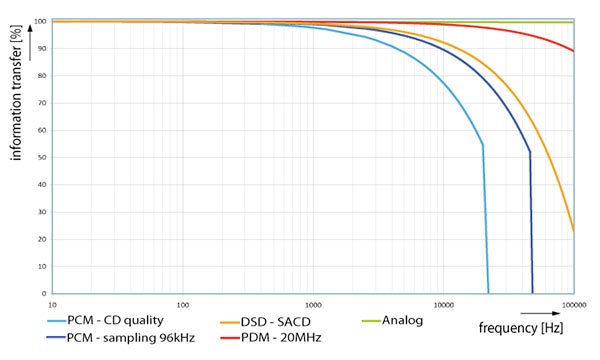
Figure 1 – A graphic showing the “information transfer of digital and analog sound systems”.
The green line at the top is perfectly horizontal indicating that no information is lost if the signal path is 100% analog. There is no mention of the myriad things that can diminish the sound quality of an analog signal (ground hum, distortion, crossover distortion etc). The graph uses this as the ideal against which the others are compared.
The Super Audio Live people (the creators of the graphic) include their 20 MHz 1-bit technology as shown on the red line. This is not a recording format and restricted to their live sound systems, so I won’t address it.
DSD – SACD, the orange line is the third best format in the illustration. The percentage of information transferred by the 1-bit 2.8224 MHz format eclipses both of the PCM formats at 44.1 (CD-Spec) and 96 kHz. They extend the line to 100 kHz, which doesn’t account for the 1-bit or 6 dB signal to noise ratio.
The important thing to notice is the curving line that starts at around 1 kHz. Why is any information lost starting at 1 kHz? Are the authors claiming that aliases that are the result of poor LPFs wrapping around the Nyquist Frequency and messing with the “information”? I get that the blue lines come to a hard stop at 22.05 and 48 kHz. Based on the sample rates of 44.1 and 96, the recordable frequency range stops right at the Nyquist Frequency or half the sample rate.
But the Low Pass Filters in the ADs are very capable of removing virtually all of the frequencies higher than Fs/2. Thus there is no gentle downward pointing curve at 1 kHz. We can rested assured that high-resolution audio recorded at 96 kHz extends the frequency range well beyond 22.05 kHz AND allows designer to avoid “brickwall” filters.